Is your problem getting worse or better? Does it fluctuate regularly or randomly? To answer these questions you need to study your problem by graphing either the number of events or a rate against time. A rate is typically the number of crime or disorder events divided by the number of targets at risk (Step 27).

The time course of a problem can be divided into three basic components:

• The overall trend, which may be obvious from visual inspection, and which shows whether the problem is getting worse, better, or staying the same over a long period.
• Seasonal, daily, and weekly cycles.
• Random fluctuations that are caused by a large number of minor influences.

Systematic study of the time course of crime is called "time series analysis."

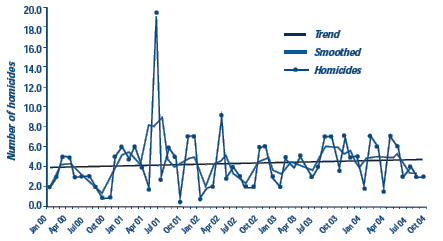
Figure 1 shows homicides in Buffalo, New York. The straight line through the middle of the chart shows the overall trend. It is virtually flat, indicating very little upward trend (though it is increasing slightly at about 1 homicide per 100 months). May 2001 was a particularly bad month, and October and November of 2000 were particularly low months.

Figure 1: HOMICIDES IN BUFFALO, NY Jan. 00 through Oct. 04

Throughout the 58 months there is considerable monthly variation, shown by the jagged peaks and valleys. Low frequency problems tend to have this characteristic, whereas problems with many events per time period often show smoother changes. These random fluctuations can hide systematic variation. One method for revealing a trend obscured by random variation is to use a moving average. This is called "smoothing". A 3-month moving average was used in this example. The July value, for example, is the average of June, July, and August while the August value is the average of July, August, and September. Notice that there is no data for the first and last months of the series because we do not have 3 months of data for these months. Moving averages fill in the valleys and knock off the peaks. Longer moving averages produce smoother graphs than shorter ones, but they can also hide useful information by making the graph too smooth.

Cycles can be detected by comparing the same months of the year (or same weeks of the month, or same days of a week, or same hours of a day, depending on the time periods you are examining). It is important to note that months are of different lengths (and do not forget February in leap years) as this might influence the number of problem events. Some analysts use 4-week periods, rather than months, to address this issue.

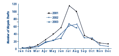
Obvious seasonal cycles can be seen in Figure 2. Here we see the number of bicycle thefts per month over 32 months. Thefts consistently peak in July and August, and consistently reach their minimum in January and February. We can also see that on a month-to-month basis 2001 was usually worse than 2002 and the months of 2003 for which we have data. This makes some sense, as there are more bicycles available to steal in the summer and even thieves have little use for bicycles in the winter (especially in Buffalo!).

Separating a time series into component parts is very useful for revealing possible causes of a problem. The homicide trend, for example, could be decomposed into two charts showing domestic homicides and non-domestic homicides (or firearm and non-firearm). So if the non-domestic homicides were trending upward while domestic homicides were declining, this would suggest that attention should be focused on non-domestic homicides.

Time series analysis is a powerful tool for evaluating the effectiveness of a response. The basic principle is to obtain a good idea of a problem's natural trends, cycles, and variation before the response is implemented, using the techniques just discussed. This tells you what you can expect from the problem in the future, if you did nothing about the problem. This provides a basis for examining time frames after the response. Changes in the trend, cycles, or even the random fluctuation suggest the response had an impact. The longer the time frames before and after, the greater the confidence you can have in your conclusions.

Time series analysis can also be very complex, so if there is a great deal depending on a precise answer to a time frame analysis, it may be useful to seek the help of a statistician specializing in this area.

Next Step

Figure 2: SEASONAL EFFECTS IN BUFFALO BICYCLE THEFTS Jan. 01 through Aug. 03