
Center for Problem-Oriented Policing
POP Center Tools Assessing Responses to Problem, 2nd Ed Page 4
Conducting Impact Evaluations
An impact evaluation has two parts. The first involves the measurement of the problem: how big is it? The second involves ways of systematically comparing changes in the problem to discover if it shrank after the response or if it shrank more than other similar but untreated problems. The second part is called the evaluation design. Evaluation designs are created to provide the maximum evidence that the implemented response was the primary cause of the change in the measure. Weak designs provide little confidence that the response caused the change. Strong designs provide much greater confidence in the conclusion that the response was the cause of the problem’s demise.
Measures
Impact evaluations require measurements of the problem before and after the response has been implemented. (Appendix B describes a commonly used bad design that does not have a before measure.) Decisions about how to measure the problem should begin at the scanning stage and be settled by the time the problem analysis has been completed. This will allow information collected during the analysis stage to be used to describe what the problem looked like before the response. During the assessment stage, measures are taken after the response has been implemented. The problem is measured the same way before and after the response.
Quantitative Measures
Measures can be qualitative or quantitative. Quantitative measures involve numbers. The number of burglaries in an apartment complex is a quantitative measure. One can count them before the response and after the response, and calculate the difference. Quantitative measures allow you to use mathematics to estimate the impact of the response. For example, burglaries went down 10 percent from before the response to after the response. In the example above, the counts of active sex workers and the traffic volume figures are both quantitative measures.
Qualitative Measures
Qualitative measures allow comparisons, but mathematics cannot be applied to them. In the example, observations of how sex workers interact with johns is a qualitative measure. Though most evaluations use quantitative measures, qualitative measures can be extremely useful. The fact that you cannot add, subtract, multiply, or divide qualitative measures does not mean they are useless. The important thing is that these measures are collected systematically and before and after the intervention so that the measures are comparable. Photos of the cleanliness of an area before and after a problem-solving effort might be useful, if they are taken at the same locations in the same lighting conditions, from the same angle and from the same distances. An arbitrary set of snapshots before and after the response is of little value in assessing the response.
Maps
Maps provide another method of qualitative measurement. Maps are very useful for showing crime and disorder patterns. Though the number of crimes is a quantitative measure, and the size and shape of the crime patterns is typically drawn using a computer algorithm, when we compare map patterns we typically use qualitative comparisons.
Measurement Validity
For both qualitative and quantitative measures, you must make sure that the measures record the problem and do not record something else. For example, counts of drug arrests are often better measures of police activity than changes in a drug problem. You should use arrest data as a measure of the problem only if you can be certain that police enforcement efforts and techniques have remained constant. On the contrary, systematic covert surveillance of a drug-dealing hotspot before and after the response could be a valid measure, if the form of surveillance was unchanged and remained undetected by the drug dealers. Measures are seldom valid or invalid; rather, they are more or less valid than alternative measures.
In short, you want to make sure that the change in the problem you measure is due to changes in the problem and not due to changes in the way you take the measures. One way of thinking about this is to compare it to physical evidence gathered at a crime scene. The reason there are strict protocols for the gathering and handling of evidence is because we do not want to confuse the activities of the offender with the activities of the evidence gatherers. The same thing is true in evaluations.
The less direct the measurement is, the less validity it has. For example, if you want to measure drug dealing, surveillance on drug-dealing sites provides direct observations of drug dealing. Arrest statistics are indirect because they involve the activities of the drug dealers and customers (the aspects of the problem you may be most interested in), as well as decisions by citizens to bring this to police attention, police decisions to intervene, and police decisions as to how they will intervene. These decisions by citizens and by the police may not always be related to the underlying reality of the problem. For example, changes in police overtime policies or the presence of special anti-drug squads can change the number of arrests, even if the drug problem remains constant. For this reason, the number of arrests of drug dealers is a less direct, and often a poor, measure of a drug problem.
Sometimes, however, it is impossible to get a direct measure of the problem and an indirect measure needs to be used. In 2004, twenty-three Chinese immigrants were drowned harvesting shellfish in the United Kingdom. A problem-solving effort was undertaken to reduce the chances of this occurring again.
Evaluating the success of the response was difficult because deaths by drowning were (fortunately) rare and multiple deaths by drowning were even less common. Therefore, counting the number of deaths by drowning before and after the effort would overestimate the success of the project, because there had been an unusually high number of such deaths in the one incident before the effort and, even if the police did nothing, there would probably be a very low number of them in the future. The police evaluators, instead, counted rescue calls to the coastal rescue service. The evidence showed that these calls declined substantially, thus providing evidence consistent with a successful response.3
Let’s return to the prostitution problem to see another example of indirect and direct measurement. In this example, the meaning of direct and indirect depends on how one defines the problem. Men drive into a neighborhood on Friday and Saturday nights looking for prostitutes to pick up. This annoys the neighbors. They call the police to do something. You have a choice of two measures for this problem.
The first is a quantitative measure taken from automatic traffic counters strategically placed on the critical streets three months before the intervention and left there until three months after the response was completed. These devices measure traffic flow. The difference between the average Friday and Saturday night traffic volume and the average volume during the rest of the week is used as an estimate of the traffic due to prostitution.
Your second measure is based on interviews of local residents taken three months before the response and three months afterwards. Residents are asked about their perceptions of the prostitution problem using a numerical scale (0 = none, 1 = minor, 2 = moderate, 3 = heavy).
If you have defined your problem as prostitution-related traffic, the first measure is a more direct measure than the second. Not all of the difference between the traffic level on Friday-Saturday and the level during the rest of the week is due to prostitution, but a large part of it probably is. So, this is a reasonable approach. Asking citizens for their perceptions, however, is fraught with difficulties. Their current perceptions of prostitution may be colored by past observations. They may not see much of the prostitution traffic, particularly if they are hiding indoors to avoid the problem. They may misperceive other activities as prostitution related.
If, on the other hand, you have defined the problem as the residents’ annoyance with prostitution-related traffic, the interviews are a more direct measure than the traffic counts. Prostitution-related traffic may have not changed, but the citizens think it has. By this measure, the response was a success. But if prostitution-related traffic (measured by the counters) has declined precipitously and the citizens are unaware of it, then, by this measure, the response has not worked.
Of course, multiple measures can be used. In this example, one could measure both the reduction in prostitution-related traffic and the perceptions of it. Only if both declined would success be unambiguous. If the traffic counters indicated a drop in traffic but the citizen surveys showed that the residents were unaware of the decline, the response could be altered to address the perceptions.
Selecting Valid Measures
How do you select specific measures for your problem? There is no one answer to this question that can be applied to any problem-solving effort. If you are working on a problem for which a problem-specific guide has been prepared, you can find some ideas for problem-specific measures listed in it. If you are working on another type of problem, the simplest approach is to use one or more of the indicators of the problem that you used to identify and analyze the problem. It is important, however, to think carefully about problem definition. As we saw in the prostitution example, seemingly minor changes in how we define the problem can have significant implications for measurement. Clearly, one needs to think about evaluation measures as soon as one begins a problem-solving process.
One way to clarify the measures to be used is to pose the question: “Why do we, the police, care about this problem?” The answers lead to outcome measures. Among other reasons, police care because: (1) citizens are annoyed (or scared); (2) people are getting hurt; (3) it’s costing the city too much money; or (4) it’s wasting police time. Note that these example answers are not generically valid. Prostitution activity in an industrial-warehouse area should produce different answers than the same activity in a residential area. Note also that “it is against the law” is not a valid answer. The law is a tool to help reduce problems, so compliance is not an outcome. Reduction in the problem is the outcome.
Criteria for Claiming Cause
As we discussed above, a problem-solving assessment has two goals: to determine whether the problem has changed, and to determine whether the response caused the change in the problem. We are particularly interested in the first goal. The second goal is only important if (1) the problem has changed, and (2) a similar response may be used to address other problems. If neither of these conditions is met, we do not need to worry about cause and the evaluation is relatively simple. If, however, the problem has changed and it is likely that the response will be used again, it is important to determine whether the response was in fact the cause of the change. If the problem decreased for reasons other than the response, then using the response again, in similar circumstances, is unlikely to produce useful results.
What if the problem has gotten worse, following the response? The response might or might not be responsible for this. If you can determine that the change in the problem was not due to the response, the response might be useful for other problems. If the response did cause the increase in the problem, you clearly do not want to use it again and should warn others not to use it.
The concept of cause may seem pretty straightforward, but it is not. Before you can confidently proclaim that a response caused the problem to decline, you need to meet four criteria. The first three criteria are relatively straightforward, and are often achievable. The fourth criterion cannot be achieved with absolute certainty. We discuss these below.
A Plausible Explanation of How the Response Reduces the Problem
The first criterion is that there must be a convincing argument showing how the response is supposed to address the problem.† This explanation should be based on a detailed analysis of the problem, preferably augmented by prior research and theory. The fact that others used a similar response and were able to reduce their problem is not an explanation. Such information is useful, but there is still a need to explain how this occurred. Absent a convincing explanation, you do not know whether this prior experience was successful by accident, whether its success was unique to the situation in which it was first applied (and will not work on your particular problem), or whether it is a generally useful response.
† The technical term for this criterion is “mechanism.”
Returning to the prostitution example, we can illustrate what is meant by a plausible explanation. We will focus on the street-pattern alterations. Police and local residents know from observations that the prostitutes congregate along a three-block stretch of roadway (between 1st and 4th streets on B Street), one block off of a very busy thoroughfare (A Street). There are traffic lights on each of the numbered streets (see Figure 3, left panel). All of the streets are two-way. The area between A and B streets largely comprises a vacant old warehouse and a light-industrial area. The prostitution activity along B Street makes use of the abandoned properties. Customers come onto B Street from A Street using the numbered streets and circle the blocks looking for women they can solicit.
Between B and C streets is an old residential neighborhood of single-family homes called the “Elms.” C Street has become a thriving entertainment and arts area, and the “Elms” is being rehabilitated as older residents sell their homes to younger, more affluent couples. Residents of the Elms complain about the traffic and noise, the harassing calls of the customers and prostitutes, and the litter of drink containers, condoms, and other debris.
To address this problem, residents have proposed a series of changes to the streets. B will be made one-way north and Elm one-way west, while 4th Street will be made one-way east between A and B streets. The other numbered streets will be disconnected from A Street and their traffic lights removed. A new traffic light will be put at the corner of Elm Street and A Street but only left turns from Elm Street onto A Street will be permitted. Another traffic light will be placed at the intersection of Elm and C streets. These changes are shown in the right panel of Figure 2.
Figure 3: Street Layout Before and After a Response to Prostitution
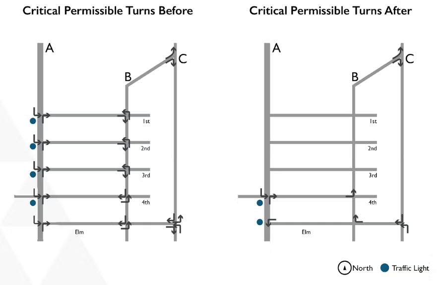
Why do the residents think this will work? We hope their answer is a plausible explanation—it is logical and takes into account the known facts. The residents claim that this area is a hotbed of prostitution activity in large part because the streets facilitate the shopping behavior of customers and the advertising displays of the prostitutes. Customers can cruise around the block quickly, looking for prostitutes. By changing the street pattern in the manner described, circular cruising becomes more time consuming. If customers do not make a contact on the first pass, they will spend much more time on the return trip. Because the customers’ convenience is reduced, fewer of them will come to the area and the problem will be reduced. In addition, once the traffic flow has been streamlined, it will be easier for the police to detect prostitution-related activities, thus increasing the risk of detection. By observing customers and prostitutes, we can verify the cruising behavior. If this explanation is logically consistent with the available information, and there is no clear and obvious contradictory information, the residents have passed the first hurdle for establishing a causal connection.
Many plausible ideas do not work when tested, so a plausible explanation by itself does not guarantee that the response will work. But it does make the response a more likely candidate for a successful solution than explanations that are not grounded in logic, fact, and experience. Prior research is important in establishing plausibility. Success of the response used in the example is made plausible by fact that previous research describes the relationship between prostitution and circular-driving patterns4 and shows that reducing the ease of traffic movement through neighborhoods sometimes reduces crime.5 Further, this intervention is consistent with the theory of Situational Crime Prevention, particularly the strategy of increasing the offenders' effort.6 Too often, police, elected officials, and the public stop at the notion of plausibility and assume that if it sounds reasonable, it must be true. And just as often, evidence demonstrates this initial hunch was wrong.
In summary, the first step in demonstrating that a response has reduced the problem is a plausible explanation of (1) how the problem operates and (2) how the response is supposed to disrupt this operation. This explanation should tell how, where, when, and why the response works. If such an explanation is prepared when the response is being crafted, it can help guide the planning and implementation of the response. The more specific this explanation is, the better the response will be and the more informative the assessment will be. Ideally, this explanation would also describe the circumstances under which the response is unlikely to work. This can aid in both the process evaluation and the impact evaluation.
The Amount of the Problem and the Level of the Response Are Related
The second criterion for claiming that a response caused a decline in the problem is that there is a relationship between the presence of the response and a decline in the problem (and the absence of the response and an increase in the problem).‡
‡ The technical term for this criterion is “association.” Typically, association is measured by the correlation between the response and the level of the problem.
Let’s go back to the prostitution problem. How would we demonstrate a relationship here? Are there similar neighborhoods that we could compare to the Elms? Just north of the Elms, there is a neighborhood like the Elms (it is also between A and C streets with a deteriorated light-industrial area to the west and the thriving C Street development to the east), but the streets do not allow easy circular-driving patterns. Now if the ease of circular driving is associated with prostitution, we should see little or no prostitution in this other neighborhood. This would imply that changing the street pattern in the Elms might be helpful. However, if there is prostitution in this area too, there is not a strong link between prostitution and ease of circular driving and this suggests that changing the street pattern may not be effective. Either way, the evidence would not be strong, but the findings could be helpful.
We might also attempt to demonstrate a relationship by measuring the problem before and after the street changes. If we see high levels of prostitution (or high levels of resident perceptions of prostitution) before the changes but low levels on these measures after the street changes, we will have evidence of a relationship.
To clear the second hurdle in claiming causation, we must demonstrate that the situation has more of the problem in the absence of the response than when the response is in place. If so, it is tempting to declare victory at this stage; however, there are two other hurdles that must be surmounted before we can be confident that the solution was responsible for the decline in the problem. This brings us to the third criterion for demonstrating a causal connection.
The Response to the Problem Comes Before the Problem’s Decline
The third criterion is that the decline in the problem comes after the response;§ logically, a response would not have an effect before it is implemented. There is one major caveat here: by response, we include publicity—intentional or accidental—about the response. A crackdown on drunk drivers may be preceded by a widespread media campaign; if so, potential drunk drivers may alter their behavior even before the intervention. In this case, the media campaign is part of the response. A decline in drunk driving after the media campaign begins but before the crackdown, could be credited to the response.† However, a decline in drunk driving prior to the media campaign would be evidence that something other than the response has caused the problem to dissipate.
§ The technical term for this criterion is “temporal order.”
† The technical term for this phenomenon is “anticipatory benefit.”
Despite its obvious simplicity, it is surprisingly common to see violations of this criterion. Throughout the 1990s homicides declined in large cities in the United States. In the middle of the decade, a couple of years into the downward trend, several U.S. cities implemented crime-reduction strategies and gained substantial notoriety. As homicides continued to decline in these cities, proponents claimed that these reductions were due to the new strategies. In point of fact, homicides had been declining prior to the changes. Because homicides were trending downward before the changes, it is difficult to attribute the decline to changes in police strategies.‡ In short, the purported cause of the decline came after the decline began. If these same changes had been implemented in 1990, the claim that they caused the drop in homicides would be more plausible.
‡ There is another reason to be skeptical that the changes in policing caused the decline in homicides. Homicides declined in other large cities that had not implemented the same changes. For a more detailed examination of the police contribution to the decline in homicides through the 1990s, see Eck and Maguire (2000).
To demonstrate that the response preceded the problem’s decline, you must know when the response began (including publicity about it) and then have measures of the problem before this time and after this time. This is called a before-after (or a pre-post) evaluation design. It is the most common evaluation design, but it is not a particularly strong design. That is, a simple pre-post design can show a decline, but it is insufficient for establishing what caused the decline.
Despite its superficial simplicity, this criterion can be difficult to demonstrate. But even if you can show that the decline in the problem came after the response, you need to achieve one more criterion before you can definitively claim that the response caused the decline: you must eliminate the alternative explanations.
Elimination of Alternative Explanations
Let’s continue with the prostitution problem. You have an explanation, you have demonstrated a relationship, and you have shown that the response came before the decline in the problem. You now need to make sure that nothing else could have caused the decline in prostitution.§ Recall that the C Street corridor and the Elms are going through a series of changes. New people are moving into the area and they are allying themselves with the remaining older residents to clean up the area. One thing they did was to call upon the police to help. Did they do anything else? Suppose the Elms’ Neighborhood Association (ENA) and the C Street Corridor Business Association (CSCBA) identified the owners of the abandoned and vacant property and put pressure on them to clean up their property. This denied prostitutes access to the property. And suppose these changes got underway about the same time the street changes were being implemented. So, one could think of the ENA and the CSCBA as the cause of the street changes and the changes in land use. If the land-use changes were the real cause of the reduction in prostitution, and the street changes were irrelevant, you would still see a relationship between the street closures and a reduction in the prostitution, and you would still see the response before the reduction. Nevertheless, something else would be responsible for the decline in the problem.
§ The technical term for this criterion is “non-spuriousness.” A spurious relationship is a false relationship: it appears that the response is causing the decline in the problem, but in reality some other factor is the cause of the decline and possibly the response, too.
Figure 4 diagrams the notion of an alternative explanation. The upper panel shows what you believe: the response caused (shown by arrow) the decline in the problem. This belief may come from a variety of valid sources. Nevertheless, something else has caused both the response and the reduction in the problem (lower panel). Here, more “something else” led to more response and, at the same time, led to a reduction in the problem.
Figure 4: Alternative Explanations
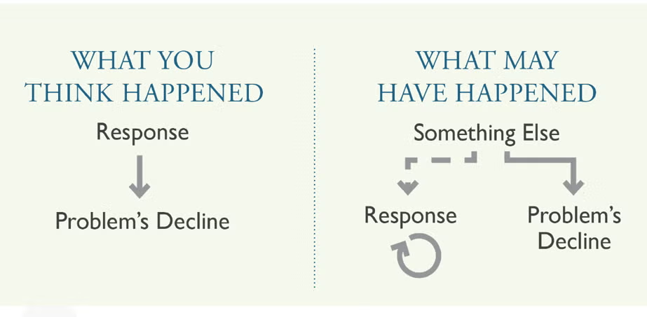
The absence of an arrow between the response and the decline in the problem means that in reality the response was irrelevant to the problem. An outsider, observing more of the response and less of the problem at the same time, might wrongly conclude that the response and problem are causally connected. In situations like this, the observed relationship between the response and the decline in the problem is misleading. The possibility of a misleading relationship between a response and a problem is a threat to the validity of an evaluation’s conclusions. Note that this is a possibility, not a demonstrated certainty. A threat to the validity of conclusions does not mean that the response was a failure. It means that we cannot be sure the response worked. There is substantial doubt because there is a plausible alternative explanation. Again, a jury trial is a useful example. If the prosecutor fails to eliminate others who could have committed the crime (and the defense brings this to the attention of the jury), the jury must have some doubts about the guilt of the defendant. Acquittal, in this case, does not mean that the prosecutor is wrong. It means that the prosecutor has not successfully eliminated alternative explanations.
There is a related concern: The “something else” might have occurred by coincidence at about the same time as your response. Practically speaking, it might not matter whether the “something else” accidentally occurred at the same time as your response or whether the “something else” caused both the response and the decline in the problem. In neither case did the response cause the drop in the problem.
To demonstrate a causal connection between the problem and the response, an evaluator needs to provide sound evidence that there is no “something else.” To accomplish this, an evaluator needs to show evidence that there are no reasonable explanations for the decline in the problem other than the response. Eliminating all alternative explanations is difficult. You can never do so definitively, because there are many possible causes of problem fluctuations. All you can do is eliminate the most obvious known alternative explanations to the decline in the problem. We can never prove that a response caused a decline in a problem, because we cannot eliminate all possible rival explanations for the decline. We can make better or worse cases for such claims, however. And this is where the evaluation design comes in. Some designs allow for stronger statements of causality than others, just as some prosecutions are more plausible to a jury than others.
Designs†
† Non-experimental designs are not addressed in this monograph because they often cannot demonstrate that the response came before the decline in the problem and because they are particularly poor at eliminating alternative explanations for the decline. Randomized designs are not addressed either. Though powerful for studying generic interventions for application across a class of problems, they are generally unsuited for operational problem solving where the primary interest is in the reduction of a specific problem rather than the testing of a generic solution. Information about these and other types of designs not described in this guide can be found in the Recommended Reading List.
An evaluation design is a systematic strategy, coordinated with the response, for organizing when and where data collection will occur. If you develop the evaluation design along with the response, the evaluation will be more likely to produce useful information. If you wait until after the response has been implemented to decide how it will be evaluated, you will have more difficulty determining whether the response was effective.
There are many types of evaluation designs that can be used (see Recommended Readings). We will discuss two common practical designs: the pre-post design (which we addressed to some extent earlier) and the time series design. Neither have control, or comparison, groups. Appendix B discusses comparison-group and multiple time series designs (the bottom row of Table 2) and describes when you might want to use a control group, or control area.
Pre-post Designs
The simplest pre-post design involves a single measurement of the problem before the response and a single measurement after the response. The after measure is compared to the before measure. If there is less of the problem after than there was before, this is evidence of a decline in the problem. As we will see, this design is sometimes adequate for determining whether the problem declined, but it is insufficient for determining that the response caused the decline.
Table 2: Types of Evaluation Designs
| Single Measurement Before and After | Multiple Measurements Before and After | |
| No Comparison (Control Group) | Pre-post design | Time series design |
| Comparison (Control) Group | Pre-post with a control group design | Multiple time series design |
Figure 5 shows results of a pre-post design. The Houston Police Department, working with the county’s mental-health authority, implemented an approach to improve the way that mentally ill people were treated. The problem-solving project was a finalist for the 2010 Herman Goldstein Award for Excellence in Problem-Oriented Policing. As part of the evaluation of the intervention, the Houston Police Department examined whether the number of mental-health-related events had declined from the year before to the year after the intervention. The pair of bars marked “total” shows that there was a substantial reduction: about 47 percent. The police also looked at the types of events—shown in the other three pairs of bars—and found that there were notable drops in all three categories.‡
‡ In most evaluation research, a test for statistical significance is used to determine whether the difference between the pre-response and the post-response is likely due to chance. In other words, one alternative explanation is that normal random fluctuations in the level of the problem caused the difference between the pre-response and post-response measures of the problem. Tests for statistical significance are most useful when the differences are small but meaningful and the number of problem events prior to the response is small. In such circumstances, normal random fluctuations in the problem are a potential cause for the change. Because of the highly technical nature of significance testing, it will not be covered in this monograph. Readers interested in significance testing can find explanations in most introductory statistics texts, in the documentation accompanying statistical software, and from statisticians and social scientists at local universities.
Such a design can establish a relationship by demonstrating that there was less of a problem when the response was present than there was when no response was present. It also helps demonstrate that the response came before the decline in the problem, because the response occurs between the two measures. However, if the level of the problem normally fluctuates, what is seen as a decline in the problem may simply be a normal low before its return to higher levels.
Variations on this simple design include making sure that the measures are taken at the same time of the year, to account for seasonal fluctuations, and using two or three pre-response measures and two or three post-response measures to account for normal fluctuations.
Figure 5: Example of Impact Measurement in a Pre-post Design

As we have seen, this design is weak at eliminating alternative explanations for the decline in the problem. This is because something else may have caused both the response and the decline in the problem, or because other things, occurring at the time of the response, may be responsible for the change in the problem.
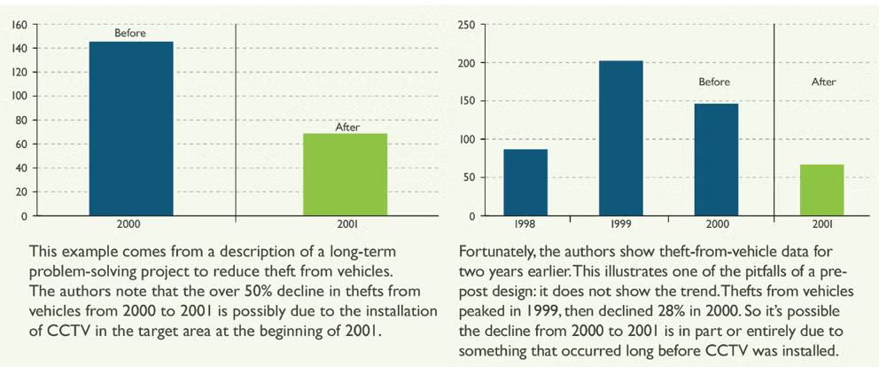
To see why a pre-post design is weak, consider the example shown in Figure 6. The data for this example come from a report on a theft-from-vehicle problem-solving effort. In the top chart of Figure 6 we see a simple pre-post comparison. The question being asked is whether the installation of CCTV in the target area caused a reduction in vehicle thefts. The answer seems to be “yes.” In the lower chart we see two more years of theft data. Two things are apparent. The downward tumble in theft-from-vehicle reports begins a year before the CCTV was installed. This calls into question the validity of a conclusion that the CCTV caused the decline. Because pre-post designs do not examine long-term trends, they cannot eliminate the alternative explanation that a decline in the problem was already underway before the intervention.
Although the pre-post design is popular, the example in Figure 6 illustrates its weaknesses. A review of the four criteria of causality makes this clear. In terms of the first criterion (that we must see a plausible explanation of how the response could reduce the problem), this simple design is no better or worse than others. In regard to the second criterion (that we must see a relationship between the response and the decline of the problem), it does not fare so well. If we compare the two panels in Figure 6, our confidence that there is a relationship between the CCTV response and thefts from vehicles goes down when two more time periods are added. Although these thefts did decline after the CCTV was added, we see that the numbers of thefts were going up and down prior to the CCTV. Problems often fluctuate, even if nothing is done about them. This means that peaks are followed by troughs, followed by peaks. Consequently, any effort implemented in a peak period will virtually be guaranteed to look good because the most likely trajectory for the problem after a peak is to go down.§ This chart raises the concern that this is what could have been going on here. We cannot be sure without more data.
§ The technical term for this “automatic process” is “regression to the mean.”
The added years of data also suggest that the third criterion (that we must be sure that the problem did not decline until after the response was applied) has been violated: thefts started going down a year before the CCTV was installed. We do not have technology that allows us to go back in time. So anytime we see a downward trend that begins before the response, we should be suspicious that the response had little or nothing to do with the decline.
Finally, the last criterion (that we need to be sure that nothing else could have caused the decline in the problem) has also not been met. Based on the data shown in Figure 6, we can imagine at least three plausible alternative explanations: (1) that thefts go up and down randomly and the CCTV was introduced while the thefts were dropping; (2) that 1999 was an unnaturally big year for thefts from vehicles, and these crimes just declined to their natural level; and (3) that some other change in the city between 1999 and 2000 created the decline (e.g., an intensive information campaign to warn drivers to remove items from the passenger compartments of their vehicles).
Figure 6: Problems With a Pre-post Design
Pre-post designs are also hard to interpret when the results indicate no change. Without knowing the long-term trend, we do not know whether the problem was trending upward before the response. If it was, and if the problem stopped getting worse following the response, then the response was successful in averting this increase. In this case, the pre-post design gives the false impression that the response was ineffective.
A final difficulty with a pre-post design is that we do not know whether the decline in the problem is sustained. Imagine that you had theft-from-vehicle data for 2002. If these data showed that there were as many thefts in 2002 as there were in 1999 or 2000, we would not be confident that the CCTV installation had made a difference. If the data showed levels of theft that were no higher than they were in 2001, we would be more confident. The longer the reduction can be maintained after the response, the more confident we are in believing that the response is working well, and that the “after” results are not some sort of fluke. It is not uncommon for programs to be successful for a short period and then the problem to bounce back after attention gets diverted to other things.
The Houston example, in Figure 5, is notable because the evaluator used multiple measures of the problem. The consistency of the drop in the problem following the response, across several different measures, gives greater validity to the conclusions. Though it is still possible that something other than the response created the declines, it is less likely that the decline is due to random fluctuations: we would not expect all measures to show the same change if randomness were the cause.
We have illustrated how the common pre-post design works, and described four concerns with interpreting the findings from such designs. All four concerns stem from not knowing the long-term trend. Next, we will examine designs that can overcome these concerns.
Time Series Designs
The time series design is far superior to the pre-post design because it can address these four concerns: there is a plausible explanation, the response is associated with a reduction in outcome, the response comes before the outcome, and the most plausible alternative explanations have been eliminated. With this design, you first take many measures of the problem prior to the response. This allows you to look at the trend in the problem before the response. It also allows you to determine the problem’s normal fluctuation prior to the response. You then take many measures of the problem after the response. This allows you to determine the long-term trend in the problem after the response. You can see whether the problem bounces back or stays down. Comparing the before trend to the after trend provides an indicator of effectiveness. This is feasible using police-reported crime data or other information routinely gathered and archived by public and private organizations. It is more difficult to accomplish if you have to initiate a special data-collection effort, such as surveys of the public.
The basic approach is to use repeated measures of the problem before the response in order to forecast the likely level of the problem after the response. If the difference between the measures taken after the response and the forecast are significant and negative, this indicates that the response was effective (see Appendix A).
This type of design provides strong evidence that the response came before the problem’s decline, because pre-existing trends can be identified. If the process for measuring the problem has not changed, this design eliminates most alternative explanations for the reduction in the problem.
Note that what matters is the number of measurement periods, not the length of time. So, for example, it is far less helpful to have three years of annual data before the response and three years of annual data after the response than to have 36 months of monthly measurements before and 36 months of monthly measurements after, even though the same amount of time has elapsed.
One might be tempted to take this to the extreme—if monthly data are better than annual data, why not weekly, daily, or even hourly data? The answer is that as the time interval becomes shorter, the number of crimes per time interval becomes too small to use for deriving meaningful conclusions. If the number of events is extremely large (as is sometimes the case when using calls-for-service data for large areas), very short intervals might be useful. But if the number of events is very small (like homicide, stranger-stranger rape, or vehicular-accident deaths in a modest-size city), one might have to use large time intervals.
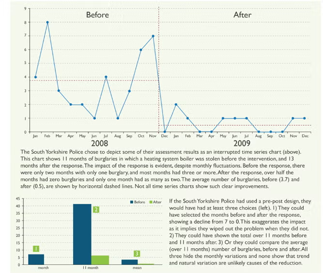
Figure 7 illustrates a simple time series design, and contrasts it to a pre-post design. This example comes from a report of the South Yorkshire Police problem-solving effort designed to combat metal theft. One form of metal theft was stealing heating boilers in residential buildings. The figure shows the frequency of such burglaries over 24 months (11 before the response and 13 after). Note the high variation in burglaries of this type prior to the intervention. A simple pre-post comparison (on the right) does not capture this, so leaves the assessment vulnerable to the problems noted earlier. It is clear from the time series chart, interrupted by the line showing when the response began, that both the number of these burglaries and the fluctuation in their numbers declined considerably, following the response. This is more convincing evidence that the trend, natural fluctuation, or lack of sustainability is unlikely to be responsible for the decline.
A comparison of the average level of the problem before and after shows a decline in the problem following the response. If the problem had been trending upward, an upward-sloping projection would have been used and the slope would have to be calculated (an example of this is illustrated in Appendix A). The more before-response time periods examined, the more confident you can be that you know the trajectory of the problem prior to the response. The more time periods examined after the response, the more confident you can be that the trajectory changed. The calculations involved in the analysis of an interrupted time series design can become quite involved; thus, if there is a great deal riding on the outcome of the evaluation, it may be worth seeking expert help.
Ideally, the only difference between the time periods before the response and the time periods after the response is the presence of the response. If this can be assured, the conclusions based on this design have a high degree of validity.
The major weakness of the interrupted time series design is the possibility that something else occurred at the same time the response began and was actually what caused the observed change in the problem. To eliminate this alternative explanation, a second time series for a control group can be added (see Appendix B).
Figure 7: Impact Measurement in an Interrupted Time Series Design
Even if you are only interested in determining whether the problem declined (and have little interest in establishing what caused the decline), an interrupted time series design is still superior to a pre-post design. This is because an interrupted time series design can show whether the problem declined and stayed down. As noted above, problems can fluctuate; thus, it is desirable to determine the stability of the decline. The longer the time series after the decline, the more confident you can be that the problem has been eliminated or is stable at a much lower level.
Though interrupted time series designs are superior to pre-post designs, they are not always practical. Here are five common reasons for this:
- Measurement is expensive or difficult.
- Data for many periods before the response are unavailable.
- Decision makers cannot wait for sufficient time to elapse after the response.
- Data-recording practices have changed, making inter-period comparisons invalid.
- Problem events are rare for short time intervals, forcing one to use fewer longer intervals.
Under these conditions, a pre-post design might be the most practical alternative.
Combining and Selecting Designs
Though we have examined these designs separately (here and in Appendix B), in many circumstances it is possible to use two or more designs to test the effectiveness of a response. This is particularly useful if you have several measures of the problem (for example, reported crime data and citizen-survey information) collected for different periods. A combination of designs selected to rule out particularly difficult to disprove alternative explanations can be far more useful than strict adherence to a single design.
Appendix C provides a structured checklist for selecting the design most appropriate for your problem. Appendix D summarizes the strengths and weaknesses of the designs discussed here and in Appendix B.
In considering what type of design or combination of designs to select, it is important to keep in mind that you cannot eliminate all alternative explanations for the reduction in the problem. Time, money, and evaluation expertise all argue for selecting the simplest design that eliminates the most obvious rival explanations. Consequently, it is useful to anticipate the most credible alternative explanations before you select an evaluation design. Once again, your analysis of the problem should give you some insight. It is also useful to listen to the most articulate critics of the response. Then, while planning the assessment, you can collect data and develop designs that address their concerns.
Examining How the Response Works
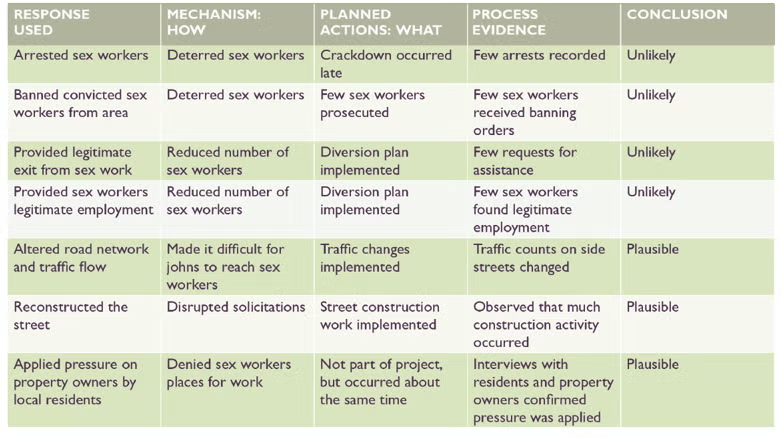
Many problem-solving responses comprise multiple parts, any of which might be effective, and some of which might not be. Further, as we noted when discussing process evaluations, sometimes parts of the response do not get implemented, or are implemented poorly. Gathering and examining evidence about implementation, as well as the plausibility of alternative explanations, helps determine what features of the response (if any) took a bite out of the problem, and which were toothless. This can be illustrated by going back to our hypothetical example of an effort to reduce street prostitution.
Table 3 lists a variety of explanations for how prostitution activity may have gone down. Such explanations are called “mechanisms.” As explained earlier, mechanisms are plausible ways in which the response could reduce the problem. Mechanisms describe how the response works. The first five mechanisms in the table are based on the planned response. The final two are mechanisms by which alternative explanations could have reduced the problem. The second column describes what happened (or failed to happen). So, for example, in the first row we see that despite the plans, not many sex workers were arrested. And in the sixth row we see that an unplanned byproduct of the street reconstruction was the presence of road workers. The third column shows the evidence supporting or contradicting the presence of the mechanism. The last column summarizes our conclusions about the likelihood that each mechanism impacted the problem.
This table shows that most parts of the planned response probably had no impact on the problem. One part may have been responsible—the street reconfiguration. Further, the table suggests that two other alternative explanations must be considered: the presence of construction crews, and the pressure from the neighbors. It also could be a combination of these three things. The construction-crew mechanism could be refuted if the prostitution activity has stayed low long after the crews have left. If it returns, however, this might be the best explanation.
Examining the response by breaking it down into its component mechanisms and examining mechanisms from rival explanations is useful if you plan to use the response again, or even if you just want to maintain the response. Here, we might stop efforts to arrest and divert sex workers. Instead, we might monitor the impact of the street reconfiguration. If we were to use this response elsewhere, we might want to proactively mobilize neighborhood residents as part of the analysis and response stages.
Table 3 illustrates a simple procedure for examining mechanisms. The first six responses deal with the planned response and its mechanism. This helps you assess which parts of the response might have worked, and which might not have. The seventh item is an alternative to the response that might have been responsible for the change in the problem. This helps you determine whether there were reasons for the change in the problem that were not planned parts of the response. Your objectives are: (1) to eliminate the least plausible mechanisms, (2) to draw a reasonable conclusion about whether the response could have caused the change, and (3) to determine what other alternative mechanisms might also have been at work. This gives you a basic assessment of what could have caused the change in the problem. It also tells you something about whether you are likely to get the same change in the problem if you use the response again. Since you usually cannot depend on the alternative explanations operating again, the more the evidence weighs in favor of these alternatives, the less likely it is that repeated use of the response will be effective.
Displacement and Diffusion of Benefits
A common concern about problem-solving responses is that they will result in spatial displacement—the shifting of crime or disorder from the target area to nearby areas that are not being treated. This concern is probably not as great as is commonly imagined.7Though displacement is far from inevitable, it is a possibility that needs to be investigated.
There is increasing evidence that some responses have positive effects that spread beyond their target areas.8 This is called “spatial diffusion of crime-prevention benefits.” Though not all responses create benefits beyond those planned for, some do, and this possibility must also be addressed in evaluations. If we do not account for these possibilities, we could produce misleading results.
We will not examine displacement or diffusion here. See Problem-Solving Tool Guide No. 10, Analyzing Crime Displacement and Diffusion, for further discussion of displacement and diffusion of benefits, how to detect them, and how to measure their impact.
Table 3: Response May Have Triggered One or More of These Mechanisms to Reduce Prostitution Activity
![]()
![]()