POP Center Tools Assessing Responses to Problem, 2nd Ed Appendix B

Appendix B: Designs With and Without Control Groups

The designs in the main body of the text focus on data for the group of people or the area receiving the response. To determine whether the response is the cause of a drop in the problem, it is helpful to use a control group. Also, control groups are critical to obtaining reasonable estimates of the amount of spatial displacement and diffusion of benefits (see Problem-Solving Tools Guide No. 10, Analyzing Crime Displacement and Diffusion). Control groups can be added to either the pre-post design or the time series design.

In this appendix, we will look at five designs, including the two examined in the body of this guide. We will use data from an evaluation of a problem-solving effort to reduce injurious and fatal vehicle crashes in Cincinnati. The evaluation used a multiple time series design and a very complex statistical
analysis process to get a precise estimate of the number of lives saved and injuries averted by implementing a response to injury-related traffic accidents. The authors found that such accidents declined 5.7 to 10.3 percent in Cincinnati compared to the comparison areas.9 This evaluation was possible because of a long-standing partnership between the Cincinnati Police Department and the University of Cincinnati’s Institute of Crime Science (based within the School of Criminal Justice).†

† Thanks to Drs. Nick Corsaro and Robin Engel of the Institute of Crime Science, within the School of Criminal Justice, University of Cincinnati, for making these data available. The Institute of Crime Science provides scientific consulting services to police and other law enforcement agencies, including complex evaluations. 

Here, we will not replicate the analysis conducted in the published paper. Instead, we will use the data to illustrate how conclusions about the effectiveness of the response can change, depending on the evaluation design used. We will start by using the data on Cincinnati traffic accidents to illustrate a design that should not be used: a static comparison group. This will be our baseline. We will then show why the pre-post design is an improvement. Then we will show why a control group is useful.
Following this, we will return to the time series design. We will conclude by showing a time series design with a control group. This brief tutorial is an introduction to evaluation designs, meant only to illustrate their basic logic.

Static Comparison Design

Let’s assume that a year after the Cincinnati Police Department’s Traffic Division launched its response, which was meant to decrease the number of injury-related traffic crashes, you are asked to determine whether it made a difference. A common design, which is not recommended, is to compare the number of injury accidents in Cincinnati to the numbers of those in nearby jurisdictions which did not use the response. The logic is that these nearby agencies would be exposed to the same traffic conditions and drivers, so they should have a similar level of accidents. That is, you are assuming that if the response worked, Cincinnati should have fewer accidents than the comparison, and that if Cincinnati had not used the response, its level of accidents would be similar to that of the comparison area.

Figure B1 shows the results. Cincinnati is contained within Hamilton County, so Hamilton County (without Cincinnati) is the comparison. Dividing the number of accidents over a 12-month period by the driving population of each jurisdiction (or road miles driven in the areas) would control for population differences. We do not do this here, for a simple reason: The principal problem with this design is that the comparison area is systematically different from the response area (they have
different driving populations, there are more highways in one area than the other, the population is older in one area than in the other, and so on). Population is just one area in which there can be many differences.

Figure B1: Static Comparison Design

You should avoid using this type of evaluation design as it has a high risk of producing misleading results. How misleading can be appreciated by comparing the results in Figure B1 to the results in the next set of figures, which illustrate better designs.

Pre-Post Without a Control Group Design

We discussed this design in the main body of the guide, so will revisit it only briefly here. Figure B2 shows the results of the evaluation of the response that was designed to lower the incidence of traffic injuries in Cincinnati. The comparison is between 12 months before the response and 12 months after. We use a full-year comparison because it controls for seasonal changes in accidents. A shorter period (e.g., the September before the response to the September after it) is highly susceptible to random changes in accidents that a response cannot address. With this design, we act as if the before measure is an accurate indicator of the number of accidents Cincinnati would have had, if no response had been applied. Therefore, the difference between the before and after measures of the problem is an indicator of the reduction due to the response.

Pre-post designs are simple. They are most useful if your principal interest is in determining whether the problem did decline and you are not going to make a strong claim that the response was a major cause of the decline.

Pre-Post With a Control Group Design‡

‡ This design is usually referred to as a “non-equivalent control group design” to draw attention to the fact that members of the treatment (response) group and members of the control group may be different in important ways that could affect the outcome of the evaluation. 

If we combine the static comparison design’s use of a control with the pre-post design’s use of a pre-response measure of the problem, we can improve the evaluation. The control area or group does not receive the response, even though it has a problem similar to that of the area or group that receives the response. The purpose of the control group is to demonstrate what would have occurred if no response had been taken. Knowing this can help you eliminate some alternative explanations for the decline in the problem.

This design is illustrated in Figure B3. Here we see that the county outside Cincinnati had a decline in injury-causing vehicle crashes from before to after the response inside Cincinnati. This indicates that even without a response, Cincinnati might have experienced a similar decline. However, Cincinnati’s decline in vehicle-injury accidents is greater than the decline in Hamilton County (over 40% greater). This indicates that the response in Cincinnati contributed to the general decline.

Figure B2: Pre-post Design

Figure B3: Pre-post with Control Design

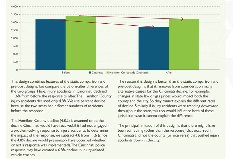
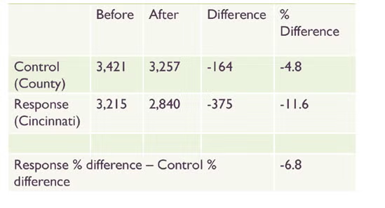
Whereas in a pre-post design effectiveness is measured by calculating the percent change, when a control group is used we compare the difference between the percent declines, as illustrated for this example in Table B1. Here we see that the control area had a reduction of 164 crashes, which, when divided by the before number (3,421), is a 4.8 percent drop. Cincinnati had a reduction of 375, which, when divided by the before number (3,215) is an 11.6 percent drop. Subtracting the percent decline in the control from the percent decline in the response yields a net reduction of 6.8 percent (dividing -6.8 by -4.8 shows that the Cincinnati drop was almost 42 percent greater than the county’s drop).

Table B1: Calculating Effectiveness with a Pre-Post with Control Design

Time Series Design

This design was also discussed in the main body of the guide. Figure B4 shows the time series for the Cincinnati vehicle crashes with injuries. The horizontal dashed lines indicate the average (mean) number of such crashes per month, before and after the response. The before data are used to determine what might have occurred in Cincinnati if no response had been made. Here a simple comparison of these averages suggests an effective response. Typically, an analyst will use a more-
complex statistical procedure to remove the effects of trends (here downward) and seasonal cycles. This gives a more-precise estimate of the impact. However, this type of analysis is far beyond what can be explained in this introductory guide.

Figure B4: Time Series Design

Multiple Time Series Designs

When two or more times series are used the design is called a multiple time series. This design can rule out most other possible alternative explanations for the change in the problem. Figure B5 illustrates a multiple time series. This example illustrates the usefulness of adding a control time series. If we had simply looked at Figure B4, we could legitimately have assumed that much of the decline in Cincinnati’s injury-related crashes could have been due to the downward trend that preceded the response. In Figure B5 we see that the trend influenced the surrounding county as well as the city. The differences in the average number of crashes per month between the city and county grew larger after the response: before, the county had an average of 35 more crashes than the city in a month; after, the county had an average of 42 more crashes than the city in a month. Like the simple time series design, analysts use highly complex statistical techniques. The study these data come from illustrates some of the complexity involved.

The principal advantage of using a multiple time series design is that it can eliminate a large number of alternative explanations for an improvement in the problem. The only possible alternative to the claim that the response caused the decline is that something occurred in Cincinnati at about the
same time as the response was implemented, and this thing did not occur in the county (or it occurred in the county but not the city). So the results of a multiple time series design, though solid, are not certain. However, for practical purposes, these results probably exceed the level of certainty we need in order to consider the response to have been successful.

Figure B5: Multiple Time Series Design