Crime Analysis for Problem Solvers in 60 Small Steps

How do you know that a response caused a problem to decline? Most problems vary in intensity, even when nothing is done about them. For example, on average there are 32 vehicle thefts per week in a particular city center, but seldom are there weeks with exactly 32 thefts. Instead, 95 percent of the weeks have between 25 and 38 thefts, and in 5 percent of the weeks fewer than 25 or more than 38 thefts are recorded. Such random variation is common. A reduction in vehicle thefts from an average of 32 per week to an average of 24 per week might be due to randomness alone, rather than a response. Think of randomness as unpredictable fluctuations in crime due to a very large number of small influences, so even if the police do nothing crime will change.

A significance test tells us the chance that a change in crime is due to randomness. A significant difference is one that is unlikely to be caused by randomness. It is harder to discern whether a small difference is significant than it is to find significance in a large difference. It is also harder to find a significant difference in a normally volatile crime problem, even if the response is effective. And it is harder to find significance if you are only looking at a few cases (people, places, events, or times) than if you are looking at many (again, even if the response was effective.) You cannot control the size of the difference or the volatility of the problem, but you may be able to collect data on more cases.

Consider the following common situation. You want to determine if crime dropped in an area following a response. You have a number of weeks of crime data prior to the response and a number of weeks of data for the same area following the response. You calculate the average (mean) number of crimes per week for each set of weeks and find that crime dropped.

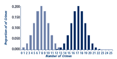
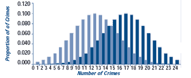
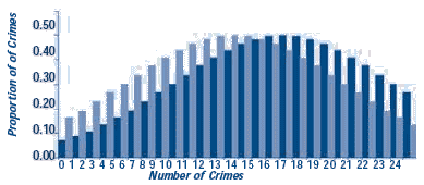
The figure shows three possible results. In each panel there are two distributions, one for the weeks before the response and one for the weeks after the response. The vertical bars in each chart show the proportion of weeks with 0, 1, 2, or more crimes (for example, in the top chart, 6 crimes occurred in 20 percent of the weeks after the response). In panel A, the distributions barely overlap because the difference in means is large and the standard deviations of the two groups are small (see Step 22). Even with a few weeks of data, a significance test could rule out randomness as a cause. In panel B, there is greater overlap in the distributions, there is a smaller difference in the means, and the standard deviations are larger. It takes many more cases to detect a non-random difference in situations like this. In panel C, there is almost complete overlap, the mean difference is even smaller, and the standard deviations are even larger. Only a study with a very large number of cases is likely to find a significant difference here. The moral is that the less obvious the crime difference, the more cases you will need to be sure randomness was not the cause of the difference.

A. Clear Difference

       Before Mean=16 Std Dev=2

       After Mean=5 Std Dev=2

B. Ambiguous Difference

       Before Mean=16 Std Dev=4

       After Mean=10 Std Dev=4

C. Probably Random Difference

       Before Mean=12 Std Dev=8

       After Mean=12 Std Dev=8

Probability theory lets us use the mean, standard deviation, and number of cases to calculate the probability that randomness is the cause of the difference. If there is less than a 5 percent chance that the problem's change was due to random fluctuations, we reject the explanation of randomness as a cause of the change. Here, 5 percent is called the significance level. In short, because the probability that randomness is the cause is below the significance level (5 percent) we "bet" that something other than randomness caused the change. Though 5 percent is a conventional significance level, you can pick a more stringent level, such as 1 percent. The more stringent the significance level you select, the greater the likelihood you will mistakenly conclude that the response was ineffective when it actually worked. This type of mistake is called a "false negative" (see Step 37). You might pick a stringent significance level if the cost of the response is so high that you need to be very certain it works.

Occasionally, analysts use a less stringent significance level, such as 10 percent. The less stringent the level you pick, the greater the possibility that you will mistakenly endorse a response that has no effect. This type of error is called a "false positive" (see Step 37). You might want to pick a less stringent level if the problem is serious, the measures of the problem are not particularly good, and you are very concerned about accidentally rejecting a good response.

There are two ways of using significance levels. In the discussion above, we used them as rejection thresholds: below the level you reject random chance and above the level you accept it as the cause. Always pick the significance level before you conduct a significance test to avoid "fiddling" with the figures to get the desired outcome.

It is better to use the significance level as a decision aid, along with other facts (problem seriousness, program costs, absolute reduction in the problems and so forth), to make an informed choice. Many sciences, such as medicine, follow this approach. If you follow this approach, use a p-value instead of the significance test. The p-value is an exact probability that the problem's change is due to chance. So a p-value of 0.062 tells you that there is about a 6 percent chance of making a false-positive error by accepting the response. This can be roughly interpreted to mean that in 100 such decisions, the decision to reject randomness in favor of the response will be wrong about six times. Whether you or your colleagues would take such a bet depends on a many things.

It is important to distinguish between significant and meaningful. "Significant" means that the difference is unlikely to be due to chance. "Meaningful" means the difference is big enough to matter. With enough cases, even a very small difference is significant. But that does not mean it is worthwhile. Significance can be calculated. Meaningfulness is an expert judgment.

The investigation of randomness can become very complex, as there are many different types of significance tests for many different situations. There are some very useful websites, as well as books, which can help you to choose among them, and there are many statistical software programs that can make the required calculations. But if there is a great deal riding on the outcome of a significance test, or a p-value, and you are not well educated in probability theory or statistics, you should seek expert help from a local university or other organizations that use statistics on a regular basis.