

The evaluation designs discussed in the body of the text focus on data for the area receiving the response. If you want to determine whether the response caused the drop in the problem, it is often helpful to use a control group. Also, control groups are critical to obtaining reasonable estimates of the amount of spatial displacement and diffusion. You can use control groups with both the pre-post and the interrupted time series designs.
† This design is usually referred to as a "nonequivalent control group design" to draw attention to the fact that members of the response group and members of the control group may be different in ways that could affect the evaluation results.
An improvement on the pre-post design is the addition of a control group. The control group does not receive the response, even though it has a problem similar to the response group's. As noted above, the purpose of the control group is to demonstrate what would have occurred, absent the response. Knowing this can help you rule out some alternative explanations for the decline in the problem.
For example, say you are concerned that a burglary decline in an apartment complex where you implemented a response may simply reflect an overall, citywide decline in residential burglary. To rule out this alternative explanation, you measure burglaries in apartment complexes similar to the one receiving the response. If the target complex had a greater reduction than the control group, you can rule out the citywide trend as a possible cause of the decline. Your confidence in your findings is directly proportional to the similarity between the response and control groups.
Figure B.1 shows an example of a pre-post design with a control group. It indicates that the response was ineffective, because the control group's problem declined more than the response group's. In other words, the control group's decline suggests that, absent a response, the problem would have declined more than it did with the response. In this example, the response made things worse.

Fig. B.1. Impact measurement in a pre-post design with a control group
A potential weakness of the pre-post design with a control group is the possibility that the differences between the response and control groups, and not the response, caused the change in the problem. In other words, the control group does not provide a valid measure of what would have happened in the response group, absent the response. For example, say you want to evaluate a response to thefts from autos parked at a shopping mall. Instead of using another mall, with a similar problem, as the control, you use the downtown central business district (CBD). Though the mall and CBD may have superficially similar problems, the parking patterns (lots vs. streets), shopping patterns (evenings and weekends vs. weekdays), street patterns (suburban vs. urban), etc., might make the CBD too different from the mall for it to be a valid control group. A better control group would be one that shares many characteristics that could contribute to thefts from autos (similar parking lots with similar security, similar shopping patterns, etc.).
A control group should share as many characteristics as possible with the response group. Ideally, they would be the same, but this is usually impossible in operational settings. Since control and response groups will be similar in some ways but not in others, in which ways should they be most similar? Obviously, the answer depends on the problem being addressed. The best control group is one that has the same type of problem and in which the response would be a plausible intervention. In other words, the explanation for how the response works (the first criterion needed to establish causality) would apply equally well to both groups.
Even under these conditions, this design may not rule out some alternative explanations. Consider the concern that automatic processes cause a decline. If the response group has an abnormally high problem level, and the control group has an abnormally low problem level, then the response group will automatically improve, and the control group will automatically get worse, regardless of the response. To rule out this alternative explanation, you need evidence that the response group did not have an abnormally high problem level, and that the control group did not have an abnormally low problem level. Another way to rule out this alternative explanation is to use a time series design. In the body of the text, we examined a simple time series. You can improve this design by adding a control time series.
When you use two or more time series, you are using a multiple time series design. This design can rule out most alternative explanations for a change in a problem. Figure B.2 illustrates a multiple time series. The fluctuating solid line represents the problem levels for the response group before and after the response. The flat solid lines represent the average pre- and post-response problem levels for that group. Though difficult to see, there is a definite decline in the average problem level after the response.
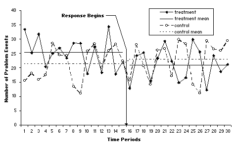
Fig. B.2. Impact measurement in a multiple time series design
The dashed lines represent the trends for the control group. The problem has slightly worsened for this group after the response. This suggests that, absent a response, the problem would not have changed, and may have gotten worse.
You may order free bound copies in any of three ways:
Online: Department of Justice COPS Response Center
Email: askCopsRC@usdoj.gov
Phone: 800-421-6770 or 202-307-1480
Allow several days for delivery.
Send an e-mail with a link to this guide.
* required
Error sending email. Please review your enteries below.


